[오승상 강화학습] 03. Markov Decision Process
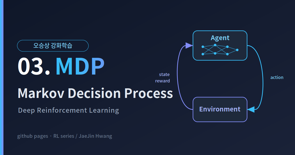
[오승상 강화학습] 03. Markov Decision Process
1. Markov Decision Process (MDP)
1-1. Markov process
- $\lbrace S_t \rbrace$ : Markov property를 만족하는 Stochastic process (collection of random variables, $S_0, \ S_1, \ \dots \ , \ S_{t-1}, \ S_{t}, \ S_{t+1}$)
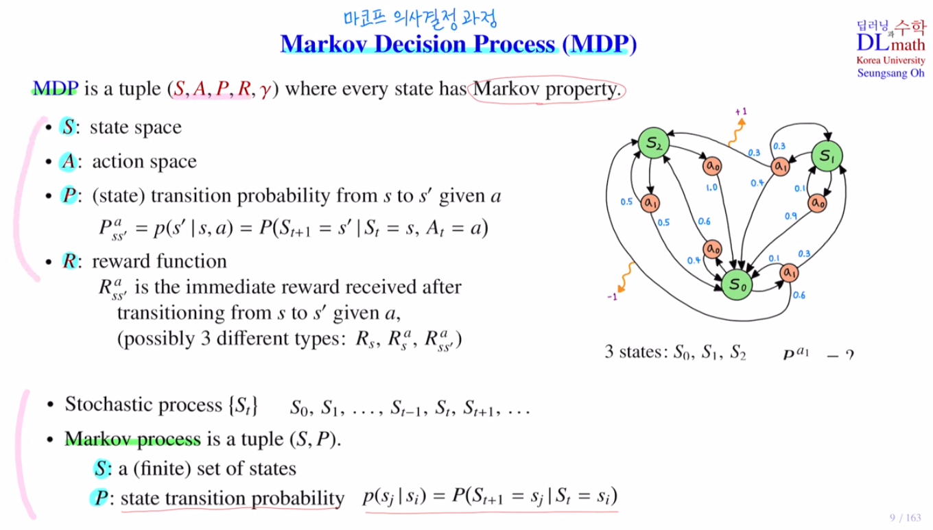
- Markov process is a tuple $(S, \ P)$
- $S$ : a (finite) set of states
- $P$ : state transition probability $P_{ij}=p(s_j|s_i)=P(S_{t+1}=s_j|S_t=s_i)$
1-2. Markov Decision Process
- MDP 이론은 $S$와 $A$가 반드시 finite할 것을 요구하지 않는다.
- 즉, state space와 action space는 continuous할 수도 있다.
- MDP는 모든 state가 Markov property를 갖는 tuple $(S, A, P, R, \gamma)$이다.
| 구성 요소 | 의미 |
|---|---|
| $S$ | state space |
| $A$ | action space |
| $P$ | transition probability |
| $R$ | reward function |
| $\gamma \in [0, 1]$ | discount factor (할인율, 0과 1 사이에 존재하는 실수값) |
$P$ : Transition probability
- $P$는 current state $S_t=s$에서 어떤 action $A_t=a$를 선택했을 때, next state가 $S_{t+1}=s^{\prime}$이 될 확률을 의미한다.
$R$ : Reward function
- $R$은 current state $S_t=s$에서 어떤 action $A_t=a$를 취해 next state $S_{t+1}=s^{\prime}$로 전이될 때 받는 reward이다.
3가지 reward type
| $R_{s}$ | 현재 state에 대한 reward |
| $R^{a}_{s}$ | 현재 state $S_t=s$ 에서 어떤 action $A_t=a$ 를 취했을 때 얻는 reward |
| $R^{a}_{ss^{\prime}}$ | 현재 state $S_t = s$ 에서 어떤 action $A_t=a$ 를 취해서 $S_{t+1}=s^{\prime}$ 로 전이될 때 얻는 reward |
1-3. MDP model example
해당 모델에서는 $\gamma$ (할인률)을 고려하지 않는다.
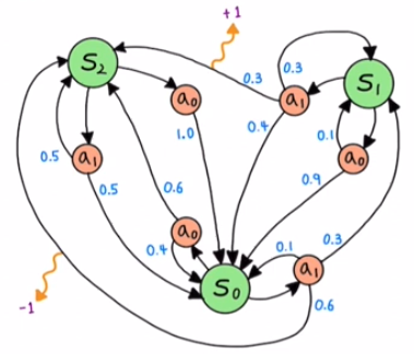
State space
- 3개의 state를 가진다. ( $S_0, \ S_1, \ S_2$)
Action space
- 2 종류의 action을 가진다. ( $a_0, \ a_1$)
Reward function
- 2 종류의 reward를 가진다. ( $+1, \ -1$ )
Transition probability example
\[P^{a_1}_{s_0 s_1} = p(s_1|s_0, \ a_1)=P(S_{t+1}=s_1|S_t=s, \ A_t=a_1) = 0.3\]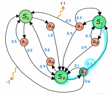
Reward function example
\[R^{a_1}_{s_1 s_2} = +1\]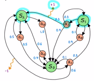
1-4. Model-based
- transition probability $P$ 와 reward function $R$ 을 알고 있을때 MDP
- model을 알고 있으므로 model 기반 문제 해결이 가능
- e.g. Dynamic programming (방대한 확률 문제를 세분화 시켜서 효율적으로 해결)
1-5. Model-free
- transition probability를 모를 때 MDP
- transition probability를 추정하지 않고, 경험(sample data)으로부터 value/Q 값을 직접 추정
- e.g. Reinforcement Learning (Q-learning, SARSA, DQN 등)
2. MDP in grid world
해당 모델에서는 $\gamma$ (할인률)을 고려하지 않는다.
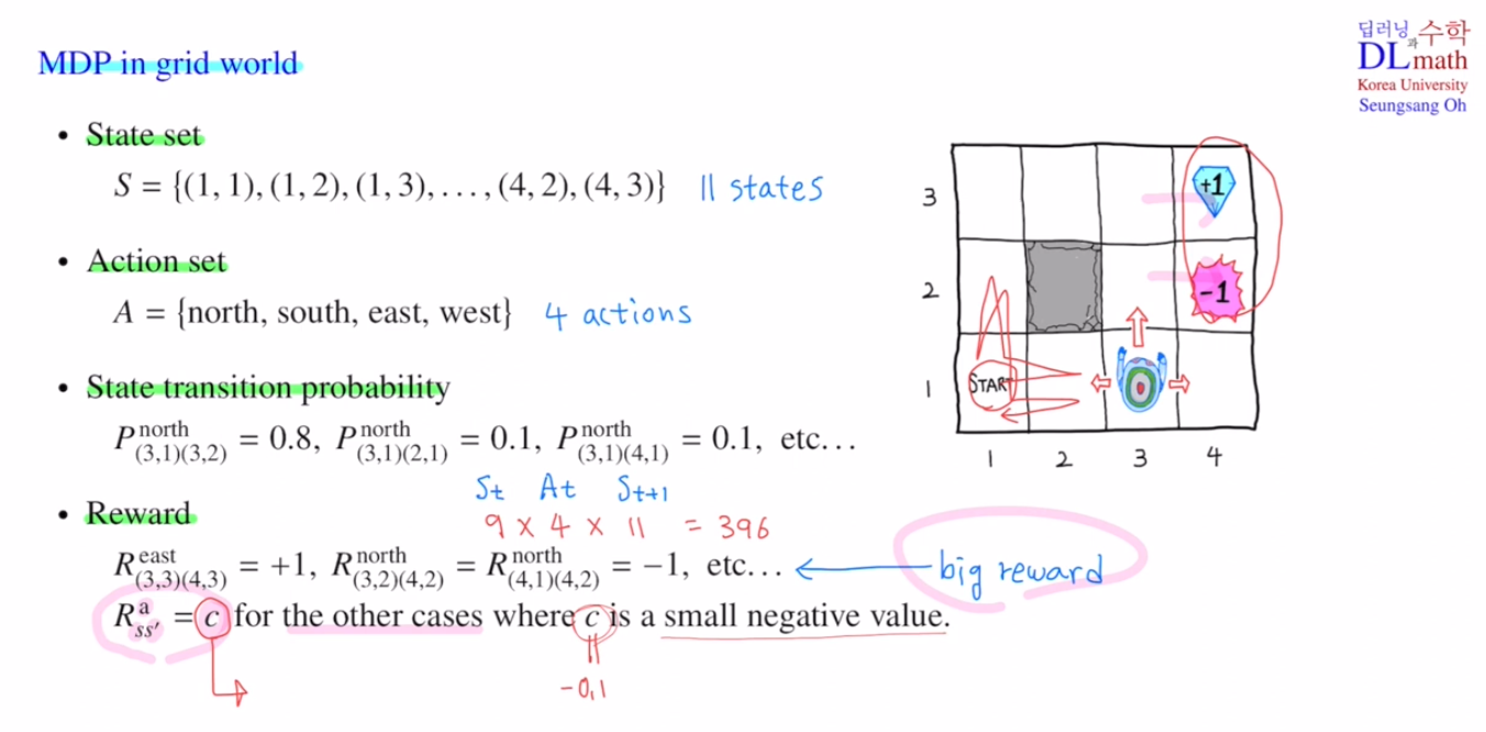
2-1. State set
- $S = \lbrace (1,1), \ (1,2), \ (1,3), \ \dots \ , \ (4,2), \ (4,3) \rbrace$
2-2. Action set
- $A =\lbrace north, \ south, \ east, \ west \rbrace$
2-3. State transition probability
\[P^{north}_{(3,1)(3,2)} = 0.8, \ P^{north}_{(3,1)(2,1)} = 0.1, \ P^{north}_{(3,1)(4,1)} = 0.1\]- Stochastic grid world 사용
- $S_t = 9$ 가지, $A_t =$ 4 가지, $S_{t+1} =$ 11 가지 ⇒ 총 396 가지 transition probability가 나오게 된다.
2-4. Big reward
$R^{\mathrm{east}}_{(3,3)\to(4,3)} = +1$ : $(4,3)$ 위치에서 마치게 되면 승점 $+1$
$R^{\mathrm{north}}_{(3,2)\to(4,2)} = -1$ : $(4,2)$ 위치에서 마치게 되면 벌점 $-1$
$R^{\mathrm{north}}_{(4,1)\to(4,2)} = -1$ : $(4,2)$ 위치에서 마치게 되면 벌점 $-1$
2-5. Small negative reward
- $R^{a}_{s s^{\prime}}$ : 한 번 action을 취할 때 마다 소량의 감점($c$) 부여
- 의미없는 action을 줄이고, 게임이 길어지는 것을 방지하기 위해서 필요하다.
3. Optimal policy in grid world
- 아래 사진의 경우, $c$ (small negative reward) 값을 각각 다르게 하였을 때의 결과로 4가지 케이스는 모두 다른 MDP model 이다.

3-1. Deterministic policy
\[\pi : S \rightarrow A, \ \ \ \ \ \ \ \ \ \ \ a = \pi(s)\]- 각 state 마다 action을 선택하는 방법
3-2. Stochastic policy
\[\pi(a \ | \ s) = P(A_t=a \ | \ S_t=s)\]- 각 state 마다 action의 확률분포를 부여하는 방법
- e.g. north(80%), east(10%), west(10%)
- 위 Grid world example에서는 stochasric policy를 적용한다.
3-3. Expected total reward
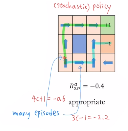
Episode
- 시작 상태 에서 출발하여 종료 상태(terminal state)에 도달할 때까지의 한 번의 완결된 경험
- policy가 정해져 있다고 하더라도, episode는 여러 개가 나올 수 있다.
- 초록색 episode의 total reward : $4c+1 = 4\cdot(-0.4)+1=-0.6$
- 파란색 episode의 total reward : $3c-1=3 \cdot(-0.4)-1=-2.2$
policy 성능 평가 방법
- policy를 평가하기 위해 한 episode가 종료된 후 total reward를 계산하게 된다.
- 이때, 일반적으로는 stochastic policy를 사용하는데, 이 경우 하나의 policy에 대해서도 여러 개의 episode가 나올 수 있다.
- 따라서, 모든 episode에 대한 total reward의 expectation(기대값)을 계산함으로써 policy를 평가하게 된다.
3-4. Optimal policy
\[\pi_*(a \ | \ s)\]- Optimal policy란, expected total reward를 maximize하는 policy
- 즉, 평균적으로 가장 좋은 reward를 받는 policy를 설정하는 것이다.
- Optimal policy는 Dynamic programming 이나 Reinforcement Learning에서 찾고자 하는 목표이다.
3-5. MDP의 궁극적인 목표
- Optimal policy( $\pi_*$)를 찾는 것
Reference
https://www.youtube.com/watch?v=S-7lXVpFci4&list=PLvbUC2Zh5oJtYXow4jawpZJ2xBel6vGhC&index=3
This post is licensed under CC BY 4.0 by the author.